Today’s post is the second that is guest-contributed by my Google Summer of Code student, Alex Kuefler. He has just finished his project on further developing Fovea, the tool for interactively investigating and analyzing complex data and models. The previous post described setting up Fovea and using it to investigate a PCA of multielectrode spike data.
As usual, and the latest version of the project source code, including the code for this post’s example, can be found on github.
Table of Contents
Introduction
In my previous post, I explored how Fovea can elucidate the process of picking the best number of dimensions to express multivariate data. As a corollary, I provided a bit of information about Principal Component Analysis (PCA) and showed off the geometry of this projection-based dimensionality reduction method. With these basics in place, we can turn to a fun application of PCA (and visual diagnostics) to a real problem in neuroscience. Namely, how do we determine which brain cells emit which spikes if we record a sample containing different signals?
Background
A multi-electrode array is a tiny bed of pin-like sensors driven into the soft jelly of the brain. Each pin (electrode) records electrical changes near individual neurons as a numerical value that dips and spikes as the cell hyper- and de-polarizes. Given that the array can contain tens or hundreds of electrodes, multi-electrode arrays collect matrix data describing voltage at many different points.
Such direct recording of many cells is sometimes likened to lowering a series of microphones into a stadium during a sports game. Whereas low-resolution brain scans (e.g., fMRI, EEG) record the roar of the entire crowd, multi-electrode arrays pick out the voices of individual neurons. But even though we can aim our recorders at individuals, we’re still bound to pick up surrounding speakers. Neuroscientists run into a problem identifying Alice the neuron, when Bob and Carol are shouting nearby.
Given waveforms recorded from electrodes at various points in a neural population, spike sorting is the process of determining which action potentials were generated by which neurons. Going from a neural waveform to a set of sorted spikes involves three basic stages:
Spike Detection Given a continuous waveform, we need to parse which peaks and troughs can really be counted as action potentials.
Feature Extraction We discriminate between Alice and Bob’s voices based on features like pitch, timbre, and word-choice. Similarly, we must decide what qualities make one cell’s spikes different than others.
Classification After detecting all the action potentials and building a profile of each one’s features, we need to leverage this information to infer which spikes (instances) were generated by which cells (classes).
Experts have a wealth of filters, classifiers, and numerical techniques for crunching through each step of a spike sort. But I’m not an expert. I like to gain insight about scary algorithms by fiddling with their knobs and seeing what happens. Fortunately, spike sorting can be visualized vividly at every step and Fovea provides the tools to do it.
Setting Up Fovea
The previous post walks through some commands for filling layers with data and slapping them over GUI subplots. The pca_disc.py code there described is an example of working with the vanilla diagnosticGUI (a global, singleton instance simply imported from graphics.py), but for a more complicate spike-sorting program, we’ll want a more personalized GUI.
Fovea now supports the option of initializing a new diagnosticGUIs to be subclassed by a user’s objects.
class spikesorter(graphics.diagnosticGUI):
    def __init__(self, title):

    #global plotter
    plotter = graphics.plotter2D()
    graphics.diagnosticGUI.__init__(self, plotter)
Instead of creating a ControlSys class to be juggled alongside the diagnosticGUI (as in pca_disc), spikesorter is a child of diagnosticGUI and can make use of all the plotting methods and attributes we’ve seen before.
In the initialization, we load in a sample waveform as a PyDSTool Pointset using importPointset() and convert it to a trajectory using numeric_to_traj(). The sample data included in the Fovea repository is a simulated neural waveform (described in Martinez, Pedreira, Ison, & Quiroga) and looks more or less like something an electrode would read out of a brain cell. For our purposes, all we need to know is that our waveform is composed from four different sources: There are two single neurons (Alice and Bob) in the immediate area of the recording channel, a cluster of nearby neurons which can’t be resolved as single cells, but whose spikes are still picked up by the electrode (multi-unit activity), and a bunch of extra-cellular noise to fuzzy things up. The end result is a waveform looking something like this:

Where the y-axis represents voltage, and the x-axis is time.
Looking at this plot, we want to determine which peaks came from Alice, which came from Bob, and which are Multi-Unit Activity from the electrode’s periphery, all while barring noise from further consideration.
Spike Detection
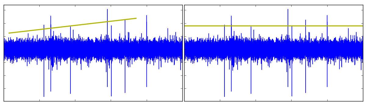
Finding true positives means admitting false positives. Such is life. When setting a threshold (i.e., the minimum acceptable height for a peak in the waveform to be considered an action potential) we invariably exclude some interesting spikes from our analysis. Or we error in the opposite direction and admit noise that’s tall enough to ride. Spike detection is a recurring theme of the last blogpost: data analysis is replete will subjective judgments, but visual diagnostics can help inform us before we make decisions.
Using Fovea’s new callbacks, we can create a threshold line to be translated up and down the waveform, admitting (or dismissing) candidate spikes as it moves along. Pressing “l” will activate line creation mode, at which point, a line_GUI object can be drawn on the axes by clicking and dragging. Once created, we can produce a perfectly horizontal threshold that extends the breadth of the data by pressing “m”.
In spikesort.py, this line won’t start detecting spikes until it’s been renamed “thresh”. Since this line_GUI is our currently selected object (having just created it), we can update its name with the following call:
ssort.selected_object.update(name = 'thresh')
At this point, pressing the “up” and “down” arrow keys will translate the threshold up and down the waveform, marking the points where it is crossed along the way.
This threshold line is best thought of as a “knob” on our analysis. We turn the knob in this or that direction and see how the tweaks propagate to our final product.
To implement special behaviors when context objects (like line_GUIs) are translated across the axes, we make use of Fovea’s new “user functions”. When we create a custom diagnosticGUI object (here called spikesorter) through subclassing, we have the option of overriding diagnosticGUI methods by defining functions of the same name. user_update_func is an example of an empty method defined in diagnosticGUI for no other reason than to be overridden. It is called every time a context object is updated. So by defining user_update_func for spikesorter, we can patch in a bit of extra behavior:
def user_update_func(self):
    #We only want the thresholding behavior to occur when 'thresh' is the updated context object.
    if self.selected_object.name is 'thresh':

        #Ensure the threshold line is horizontal by checkking for 0 slope.
        if self.selected_object.m != 0:
            print("Make 'thresh' a horizontal threshold by pressing 'm'.")
            return

        #The numeric value of the threshold is 'thresh's y-intercept.
        cutoff =  self.selected_object.b

        traj_samp = self.traj.sample()['x']
        r = traj_samp > cutoff
        above_thresh = np.where(r == True)[0]

        spike = []
        spikes = []
        crosses = []

        #Recover list of lists of points on waveform above the threshold line.
        last_i = above_thresh[0] - 1
        for i in above_thresh:
            if i - 1 != last_i:
                crosses.append(i)
                #Return x value of the highest y value.
                spikes.append(spike)
                spike = []
            spike.append(i)
            last_i = i

        self.traj_samp = traj_samp
        self.crosses = crosses
        self.spikes = spikes

        self.plotter.addData([self.crosses, [cutoff]*len(self.crosses)], layer='thresh_crosses',
            style='r*', name='crossovers', force= True)

        self.show()
Once the threshold is positioned where we want it, the “d” key will detect spikes by locating each local maximum to the right of a cross-over. These maxima are the peaks of the action potentials and each is centered in its own box_GUI object created by spikesort.py.
Unlike the “l” hot key, “d” is specific to our application. By writing a key handler method and attaching it to the canvas with mpl_connect, it is easy to patch in new hot keys like this one. However, you must be careful not to reuse function names from Fovea, as they will be overridden. The following method is named ssort_key_on (as opposed to key_on, used in diagnosticGUI) so that new key presses will be added to the old library of hot keys, rather than replacing it:
def ssort_key_on(self, ev):
    self._key = k = ev.key  # keep record of last keypress
    fig_struct, fig = self.plotter._resolveFig(None)

    if k== 'd':
        #Draw bounding boxes around spikes found in user_update_func.
        spikes = self.spikes
        self.X = self.compute_bbox(spikes)

        self.default_colors = {}

    #Draw the spike profiles in the second subplot.
    if len(self.X.shape) == 1:
        self.default_colors['spike0'] = 'k'
        self.addDataPoints([list(range(0, len(self.X))), self.X], layer= 'detected',
            style= self.default_colors['spike0']+'-', name= 'spike0', force= True)

    else:
        c= 0
        for spike in self.X:
            name = 'spike'+str(c)
            self.default_colors[name] = 'k'
            self.addDataPoints([list(range(0, len(spike))), spike], layer= 'detected',
                style= self.default_colors[name]+'-', name= name, force= True)
            c += 1

    self.plotter.auto_scale_domain(xcushion = 0, subplot = '12')
    self.show()
Once the threshold is positioned where we want it, the “d” key will detect spikes by locating each local maximum to the right of a cross-over. These maxima are the peaks of the action potentials and each is centered in its own box_GUI object created by spikesort.py.
Each box_GUI captures 64 milliseconds of neural data by default, but this value can be changed in the spikesort GUI itself. Just press “b” to create your own box_GUI, give it the name “ref_box”, and the program will use its width as the new size for detecting spikes. This trick can be used in conjunction with the toolbar zoom to make very narrow bounding boxes to fit your detected spikes.
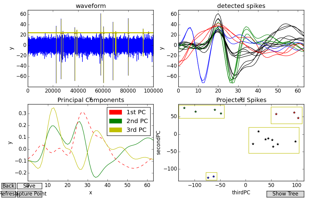
The boxes’ contents are shown in the second (“detected spikes”) subplot, as a succession of spike profiles laid on top of each other. This plot will give you a general sense of the action potentials’ shapes (and their diversity), but it’s not yet clear how to sort them.
Feature Extraction
Any given object of study can be decomposed into features in an infinite number of ways. A birdwatcher confronting a strange specimen can consider anything from the animal’s tail-plumage, to its birdsong, to the motion of its flight in order to identify it. There is no single “right” feature or set of features to look at, because the bird is a whole of many parts. Nevertheless, selecting some attributes over others and describing experimental objects as vectors across these attributes can be very useful. This process, called features extraction, discretizes nature and helps us make decisions in the face of ambiguity.
Traditionally, researchers use their domain knowledge of the subject they study to select the attributes they think are most informative. For neuroscientists, such features might be the duration or the amplitude of a spike. But Alice and Bob are closely situated in the brain. Their signals are visually abstract and more similar to one another than the appearances of crows and condors. In other words, eyeballing these spike profiles and pointing to different qualities that “seem useful” for grouping them could easily lead us astray. Is there some hidden set of features that will give us a better handle on microelectrode data? If so, how do we find it?
Alarm bells should now be ringing in the heads of PCA enthusiasts. In the last post, I described the dilemma of a psychologist who wants to find the minimum, component feelings one might use to describe all emotions. Once this set is found, any complex emotion might be described as a weighted sum of these components (e.g., “nostalgia” might decompose to 0.8*sorrow + 0.7*happiness – 0.3*anger). PCA comes up with these components by finding a set of orthogonal directions through the data that capture the greatest amount of variance. Here, “orthogonal” essentially means that no component contains even a smidgen of another component (e.g., happiness is zero parts anger and zero parts sorrow) and “greatest amount of variance” means no other components can be composed to give a more accurate reconstruction of the data than those found by PCA (assuming the components are orthogonal). By using components as our attributes, PCA acts as an automatic feature extractor driven by mathematics, rather than intuitions.
We neuroscientists with our spikes are now in an analogous situation to the psychologist. The difference here being the components PCA finds for our data will be a little more abstract and a little less amenable to an English-language description. Fortunately, we don’t need English-language descriptions of the components, because we have Fovea: We can visualize what spike components look like in the third subplot.
Pressing “p” after detecting a set of spikes will cause spikesort to carry out PCA on the n x m observation matrix whose rows are the waveform segments detected with the “d” key-press, and whose columns are the current voltages of every spike at a given time-step. PCA gives us an m x 3 projection matrix, whose columns are the principal components (PC). These PCs are displayed in the third subplot in red, green, and yellow respectively. Meanwhile, the spikes projected onto the first and second PC are shown in the fourth subplot.
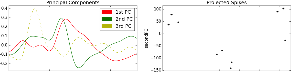
The important thing to notice about the PCs in the third subplot is that they look a bit like action potentials. Sure, no single one of them seems quite like it would fit in with the spikes of the “detected” plot. But it’s easy to imagine how, say, hammering out a few bumps in the red PC or flipping the green PC upside down and merging them together might give us one of the black spike profiles shown. Indeed, this is what the projection step of PCA is doing. Recall that each observed instance (a spike) is a weighted combination of the components (e.g., spike1 = 0.5*pc1 – 0.8*pc2 + 0.2*pc3). These weights stretch and flip the PCs in the manner above described before merging them through summation. In this sense, a PC might be described as a “proto-spike”: The wavy red, green and yellow lines don’t correspond to anything we’ve really recorded the brain doing, but they can be combined in different ways to generate any of the real spikes we did observe.
The fourth subplot, “Projected Spikes”, can be interpreted as a graph of the weights used to scale the PCs. In the below image, we use Fovea’s new picker tools to select a data-point in the fourth subplot, which highlights its corresponding detected spike as well. The chosen point is at approximated -230 on the x-axis (the red PC) and +40 on the y-axis (the green PC).
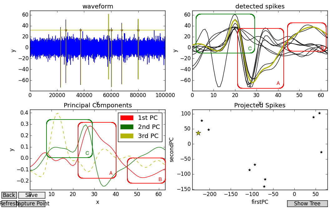
In other words, this spike contains a LOT of first PC (except flipped upside-down, as the weight is negative), and a fair amount, but substantially less of the second PC. This finding accords with intuition, as the big peak of the red PC looks like an inversion of the spike’s V-shaped refractory period (see my overlaid box A, which is not part of the Fovea output), and they both share a trough or hill at the end (see: B). Similarly, the flat onset and high peak of the spike resemble the first third of the green PC (see: C).
You may also notice that only the first and second PCs are fully drawn in, whereas the third is dotted out. This indicates the first and second PCs are being used as the axes of the fourth subplot. By clicking on the dotted PC, the user can change the projection axes of the “Projected Spikes” subplot. Below we see the same selected spike, but shown on new axes:

Classification
Two differences should stand out when projecting onto the first/second PCs rather than the second/third PCs. First, the data projected onto the first/second PCs should have a greater tendency to cluster.

Second, when we introspect these clusters they should tend to be more cohesive than groupings that show up when projecting to the second/third PCs. In other words, if we look at only those detected spike profiles that go along with a given cluster, they should all look pretty similar to one another. We use a combination of key-presses and context objects to facilitate this process. Pressing “b”, we create box_GUIs in the fourth subplot to fit around potential clusters of data point. When one of these bounding boxes is selected (in bold), we can then press either “1”, 2”, or “3” to color the points in that box red, green or blue, respectively (“0” returns them to black). The detected spike profiles will receive the new colors as well. Below, we see a few clusters grouped in this way:
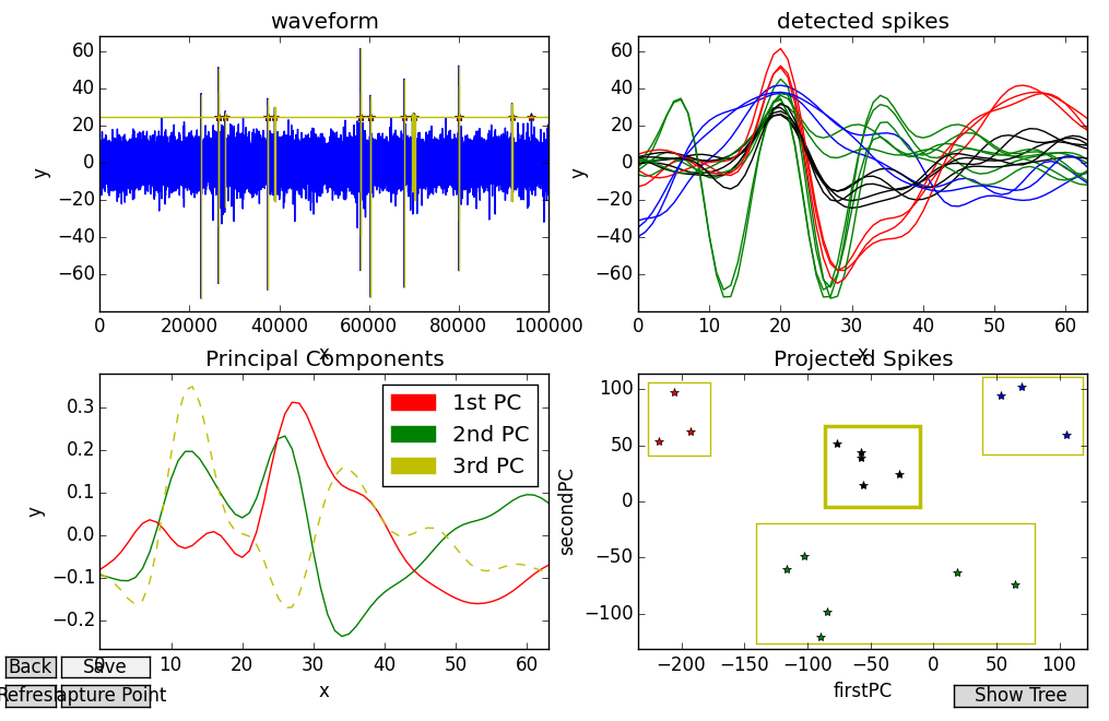
Here, four distinct clusters have been picked out and they’re all fairly easy to describe. The red spikes look like “classic” action potentials, characterized by a flat onset, high peak, and slow return to baseline. The green spikes start out with a sharp V-shape and have a distinctive, yet lower peak. The blue spikes are characterized by single, smooth swells. And finally, the black spikes always manage to cross the mean of the data, and are perhaps just noise or multi-unit activity.
On the other hand, projecting data onto the third/second PCs is less clean. Not only do the clusters seem less distinctive, but the spike profiles they group together don’t appear to have very much in common:
My placement of rectangular bounding boxes using Fovea’s “b” command in this projection was more arbitrary, as these clusters weren’t as clearly separated. Although some of the colorations accord with what we’d expect, in this projection the difference between the high-peaked “classic” spikes and the multi-unit noise we picked out from the previous example doesn’t come across (both are painted in black and belong to the large, blurry cluster in the middle). However, this projection isn’t entirely without merit. Consider the blue and green spikes. In the previous example, these were all bunched together into the same group. But it’s clear from this projection that although both sets have a distinctive V shape, for one group they precede the peak, and for the other, they follow it.
Although the literature on classification algorithms is extensive, the fact that we can turn the different “knobs” provided by Fovea and come up with unexpected results suggests the benefits of visualization for exploratory analysis.
Conclusion
In addition to exploring a real-world use case, this post lays out lots of new Fovea tools resulting from our work during Google Summer of Code 2015. We’ve seen how subclassing diagnosticGUI can produce more complicated programs and let us tailor Fovea’s behavior with user function overrides. We also took a look at built-in key presses, picking selected objects with the mouse-clicks, and some applications for the line_GUI and box_GUI context objects.
Links
Realistic simulation of extracellular recordings